
2010 Ejercicios 2: Funciones de una variable
De Software Libre para la Enseñanza y el Aprendizaje de las Matemáticas (2010-11)
Funciones a utilizar: if...then...else, assume, limit, forget, plot2d, diff, define, solve, trigexpand, trigsimp y subst.
Ejercicio 1
Sean <math>a</math> y <math>b</math> dos números reales. Se considera la función <math>f</math> definida sobre los números reales por
- <math>
f(x)=\left\{ \begin{array}{lll}
 \dfrac{e^x-1}{x}  &\mbox{si} & x>0\\
 a\,x+b           &\mbox{si} & x\leq 0
\end{array} \right. </math>
Ejercicio 1.1
Definir la función <math>f</math> usando el condicional if ... then ... else.
(%i1) f(x):= if(x>0) then (%e^x-1)/x else a*x+b$
Ejercicio 1.2
limit no puede evaluar expresiones del tipo if...then. Por ello, para determinar el límite de <math>f</math> en cero por la derecha se necesita precisar en qué intervalo se encuentra <math>x</math>. Esto puede hacerse con la función assume.
Escribir la expresión assume(x>0), después calcular el límite de <math>f</math> en cero por la derecha. Se puede eliminar la hipótesis sobre <math>x</math> con forget(x>0).
(%i1) assume(x>0);
(%o1) [x>0]
(%i2) limit(f(x),x,0,plus);
(%o2) 1
Ejercicio 1.3
Deducir el valor de <math>b</math> para el que <math>f</math> es continua en <math>\mathbb{R}</math>.
(%i1) j(x):=a*x+b $
(%i2) limit(j(x),x,0,minus);
(%o2) b
(%i3) b:1 $
(%i4) b;
(%o4) 1
Ejercicio 1.4
Calcular la derivada de <math>f</math> en cero por la derecha.
(%i1) g(x):= (exp(x)-1)/x;
(%i2) diff(g(x),x);
(%o2) %e^x/x-(%e^x-1)/x^2
(%i3) ratsimp(%o2);
(%o3) ((x-1)*%e^x+1)/x^2
(%i4) define (h(x), %o3);
(%i5) limit(h(x),x,0,plus);
(%o5) 1/2
 OTRA FORMA

(%i1) assume(x>0);
(%o1) [x>0]
(%i2) diff(f(x),x);
(%o2) %e^x/x-(%e^x-1)/x^2
(%i3) limit (%o2,x,0,plus);
(%o3) 1/2
Ejercicio 1.5
Calcular el valor de <math>a</math> para el que <math>f</math> es derivable en cero.
(%i6) j(x):=a*x+b;
(%i7) diff(j(x),x);
(%o7) a
(%i8) define (k(x), %o7)$
(%i9) limit (k(x),x,0,minus);
(%o9) a
(%i10)a:%o5;
(%i11) a;
(%o11) 1/2
Ejercicio 2
Sea <math>g</math> la función real definida por <math>g(x) = 2x-\sqrt{1+x^2}</math>
(%i1)g(x):= 2*x-sqrt(1+x^2)$
Ejercicio 2.1
Calcular los límites de <math>g</math> en más y menos infinito.
(%i2)limit(g(x), x, inf);
(%o2)inf
(%i3)limit(g(x), x, minf);
(%o3)-inf
Ejercicio 2.2
Dibujar la gráfica de la función <math>g</math>.
(%i1) g(x):= 2*x-sqrt(1+x^2)$
(%i2) wxplot2d(g(x), [x,-5,5], [y,-5,5]);

Ejercicio 2.3
Calcular <math>g'(x)</math>.
(%i1)g(x):= 2*x-sqrt(1+x^2)$
(%i2)'diff(g(x),x)=diff(g(x),x);
(%o1) 'diff((2*x-sqrt(x^2+1)),x,1)=2-x/sqrt(x^2+1)
Ejercicio 2.4
Resolver la ecuación <math>g(x)=0</math>.
(%i1)g(x):= 2*x-sqrt(1+x^2)$
(%i2)find_root(2*x=sqrt(1+x^2),x,-100,100);
(%o1)0.57735026918963
Ejercicio 2.5
Determinar los intervalos de crecimiento de <math>g</math>.
(%i1) define(w(x),diff(g(x),x))$
(%i2) find_root(w(x),x,-1000,1000)

Obtenemos el resultado:
function has same sign at endpoints
[f(-1000.0)=2.999999500000375,f(1000.0)=1.000000499999625]
 -- an error.  To debug this try debugmode(true);

Que nos indica que la función no tiene ceros en ese intervalo. Si los límites en menos infinito y más infinito coinciden con esos
valores, la derivada segunda no se anula nunca, con lo que su valor es siempre positivo y, por tanto, la función es siempre creciente:

(%i3) limit(w(x), x, inf)
(%o3) 1
(%i4) limit(w(x), x, minf)
(%o4) 3

Efectivamente, la función f(x) es siempre monótona creciente.
Ejercicio 2.6
Calcular las ecuaciones reducidas de las asíntotas de <math>g</math>.
Para comprobar si la función tiene asíntotas horizontales:
(%i1) limit(2*x-sqrt(1+x^2), x, inf);
(%o1) inf
De tener asíntota oblicua, vendrá dada por la ecuación y=m*x+n
Para calcular la pendiente de la asíntota oblicua:
(%i2) limit((2*x-sqrt(1+x^2))/x, x, inf);
(%o2) 1
Para calcular la ordenada de la asíntota oblicua:
(%i3) limit((2*x-sqrt(1+x^2))-x, x, inf);
(%o3) 0
Por lo que la función no tiene asíntotas horizontales (%o1) y la ecuación de su asíntota oblicua es y=x
Ejercicio 3
Ejercicio 3.1
Desarrollar <math>cos(3t)</math> en función de <math>cos(t)</math>.
(%i1)wxplot2d([['parametric, cos(t), cos(3*t), [t, -10, 10], [nticks, 300]]], [x,-2,2], [y,-2,2])$
(%o1)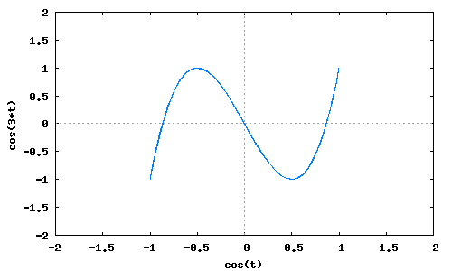

Ejercicio 3.2
Desarrollar <math>cos(4t)</math> en función de <math>cos(t)</math>
(%i2)wxplot2d([['parametric, cos(t), cos(4*t), [t, -10, 10], [nticks, 300]]], [x,-2,2], [y,-2,2])$
(%o2)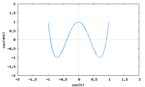

Ejercicio 3.3
Desarrollar <math>cos(5t)</math> en función de <math>cos(t)</math>.
(%i3)wxplot2d([['parametric, cos(t), cos(5*t), [t, -10, 10], [nticks, 300]]], [x,-1,1], [y,-1.5,1.5])$
(%o3)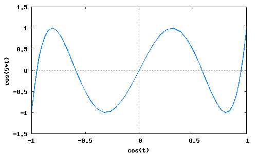

Ejercicio 3.4
Determinar los polinomios <math>T_n</math> de la variable <math>x</math> tales que para todo <math>t \in \mathbb{R}</math>, <math>cos(nt) = T_n(cos\ t)</math> para <math>n \in \{3,4,5\}</math>.
Ejercicio 3.5
Representar las funciones <math>T_3</math>, <math>T_4</math> y <math>T_5</math> en la misma gráfica.